2 Acceleration algorithms
2.1 Newton acceleration
Here we will define $g(x) = f(x) - x$. The general approach is to solve $g(x)$ with a rootfinder. The $x$ that provides this root will be a fixed point. Thus after two iterates we can approximate the fixed point with:
\[x_{i+1} = x_i - \frac{g(x_i)}{g^\prime(x_i)}\]
FixedPointAcceleration.jl approximates the derivative $g^\prime(x_i)$ so that we use an estimated fixed point of:
\[\text{Next Guess} = x_i - \frac{g(x_i)}{ \frac{ g(x_i) - g(x_{i-1})}{x_i-x_{i-1}} }\]
The implementation of the Newton method in this package uses this formula to predict the fixed point given two previous iterates.[1] This method is designed for use with scalar functions.
2.2 Aitken acceleration
Consider that a sequence of scalars $\{ x_i \}_{i=0}^\infty$ that converges linearly to its fixed point of $\hat{x}$. This implies that for a large $i$:
\[\frac{\hat{x} - x_{i+1}}{\hat{x} - x_i} \approx \frac{\hat{x} - x_{i+2}}{\hat{x} - x_{i+1}}\]
For a concrete example consider that every iteration halves the distance between the current vector and the fixed point. In this case the left hand side will be one half which will equal the right hand side which will also be one half.
This above expression can be simply rearranged to give a formula predicting the fixed point that is used as the subsequent iterate. This is:
\[\text{Next Guess} = x_{i} - \frac{ (x_{i+1} - x_i)^2 }{ x_{i+2} - 2x_{i+1} + x_i}\]
The implementation of the Aitken method in FixedPointAcceleration.jl uses this formula to predict the fixed point given two previous iterates. This method is designed for use with scalar functions. If it is used with higher dimensional functions that take and return vectors then it will be used elementwise.
2.3 Epsilon algorithms
The epsilon algorithms introduced by Wynn (1962) provides an alternate method to extrapolate to a fixed point. This documentation will present a brief numerical example and refer readers to Wynn (1962) or Smith, Ford & Sidi (1987) for a mathematical explanation of why it works. The basic epsilon algorithm starts with a column of iterates (column B in the below figure). If $i$ iterates have been performed then this column will have a length of $i+1$ (the initial starting guess and the results of the $i$ iterations). Then a series of columns are generated by means of the below equation:
\[\epsilon_{c+1}^r = \epsilon_{c-1}^{r+1} + (\epsilon_{c}^{r+1} - \epsilon_{c}^{r})^{-1}\]
Where $c$ is a column index and $r$ is a row index. The algorithm starts with the $\epsilon_0$ column being all zeros and $\epsilon_1$ being the column of the sequence iterates. The value in the furthest right column ends up being the extrapolated value.
This can be seen in the below table which uses an epsilon method to find the fixed point of $\cos(x)$ with an initial guess of a fixed point of $1$.
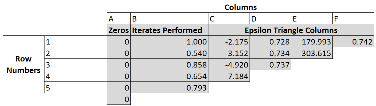
In this figure B1 is the initial guess of the fixed point. Then we have the iterates $B2 = \cos(B1)$, $B3 = \cos(B2)$ and so on. Moving to the next column we have $C1 = A2 + 1/(B2-B1)$ and $C2 = A3 + 1/(B3-B2)$ and so on before finally we get $F1 = D2 + 1/(E2-E1)$. As this is the last entry in the triangle it is also the extrapolated value.
Note that the values in columns C and E are poor extrapolations. Only the even columns D,F provide reasonable extrapolation values. For this reason an even number of iterates (an odd number of values including the starting guess) should be used for extrapolation. FixedPointAcceleration.jl's functions will enforce this by throwing away the first iterate provided if necessary to get an even number of iterates.
In the vector case this algorithm can be visualised by considering each entry in the above table to contain a vector going into the page. In this case the complication emerges from the inverse - there is no clear interpretation of $(\epsilon_{c}^{r+1} - \epsilon_{c}^{r})^{-1}$ where $(\epsilon_{c}^{r+1} - \epsilon_{c}^{r})$ represents a vector. The Scalar Epsilon Algorithm (SEA) uses elementwise inverses to solve this problem which ignores the vectorised nature of the function. The Vector Epsilon Algorithm (VEA) uses the Samuelson inverse of each vector $(\epsilon_{c}^{r+1} - \epsilon_{c}^{r})$.
2.4 Minimal polynomial algorithms
FixedPointAcceleration.jl implements two minimal polynomial algorithms, Minimal Polynomial Extrapolation (MPE) and Reduced Rank Extrapolation (RRE). This section will simply present the main equations but an interested reader is directed to Cabay & Jackson (1976) or Smith, Ford & Sidi (1987) for a detailed explanation.
To first define notation, each vector (the initial guess and subsequent iterates) is defined by $x_0, x_1, ...$ . The first differences are denoted $u_j = x_{j+1} - x_{j}$ and the second differences are denoted $v_j = u_{j+1} - u_j$. If we have already completed $k-1$ iterations (and so we have $k$ terms) then we will use matrices of first and second differences with $U = [ u_0 , u_1 , ... , u_{k-1} ]$ and $V = [ v_0 , v_1, ... , v_{k-1} ]$.
For the MPE method the extrapolated vector, $s$, is found by:
\[s = \frac{ \sum^k_{ j=0 } c_j x_j }{ \sum^k_{j=0} c_j }\]
Where the coefficient vector is found by $c = -U^{+} u_k$ where $U^{+}$ is the Moore-Penrose generalised inverse of the $U$ matrix. In the case of the RRE the extrapolated vector, $s$, is found by:
\[s = x_0 - U V^+ u_0\]
2.5 Anderson acceleration
Anderson (1965) acceleration is an acceleration algorithm that is well suited to functions of vectors. Similarly to the minimal polynomial algorithms it takes a weighted average of previous iterates. It is different however to these algorithms (and the VEA algorithm) in that previous iterates need not be sequential but any previous iterates can be used.
Consider that we have previously run an N-dimensional function M times. We can define a matrix $G_i = [g_{i-M} , g_{i-M+1}, ... , g_i]$ where $g(x_j) = f(x_j) - x_j$. Each column of this matrix can be interpreted as giving the amount of ``movement'' that occurred in a run of the function.
Now Anderson acceleration defines a weight to apply to each column of the matrix. This weight vector is M-dimensional and can be denoted $\{\mathbf{\alpha} = \alpha_0, \alpha_1, ... , \alpha_M\}$. These weights are determined by means of the following optimisation:
\[\min_\mathbf{\alpha} \vert\vert G_i \mathbf{\alpha} \vert\vert_2\]
\[\hspace{1cm} s.t. \sum^M_{j=0} \alpha_j = 1\]
Thus we choose the weights that will be predicted to create the lowest ``movement'' in an iteration.
With these weights we can then create the expression for the next iterate as:
\[x_{i+1} = \sum_{j=0}^M \alpha_j f(x_{i-M+j})\]
The actual implementation differs from the proceeding description by recasting the optimisation problem as an unconstrained least squares problem (see Fang & Saad 2009 or Walker & Ni 2011) but in practical terms is identical.
- 1Only two rather than three are required because we can use $x_{i+1} = f(x_i)$ and $x_{i+2} = f(x_{i+1})$.